Implementing Image Processing Algorithms

Throughout the past semester, as part of my computer vision course, I had to implement several image processing and computer vision techniques and algorithms to operate on grayscale images. There were three programming tasks in total. The first was to count the number of objects in a particular image, which required several simple steps. The second was to implement an edge detection algorithm, specifically Canny edge detector. The last programming assignment was to implement photometric stereo. This post will contain three (mostly) independent sections describing each of the assignments.

Counting Objects in an Image

The first assignment was to count the number of objects that were in a particular image. The image in question was a grayscale image with a very light background and approximately 1500 dark gray circles (based on the output of my program). The circles were irregular, both in color and shape, and many of the objects were touching or overlapping. Unfortunately I am unable to provide the image in question, which I will refer to as the test image.

This task was broken down into three steps. First, the image was converted to a binary image (which is just an image where each pixel is either black or white) using Otsu’s method to find the threshold. Next the image was eroded to separate overlapping components. Lastly, I performed connected-component labeling to get my final answer.

Grayscale to Binary

In order to convert a grayscale image to a binary image, you must first find the threshold which divides the light and dark areas. The threshold is a number such that any pixel with a grayscale value less than the threshold will become black in the binary image, and pixels with a value greater than the threshold will become white in the binary image. Selecting the threshold could be done manually, but it would be nice if an appropriate threshold could be automatically selected for any grayscale image. This is where Otsu’s method comes to the rescue.

Otsu’s method will automatically select a threshold based on the histogram of the image. A histogram is a chart representing the number of occurrences of different values. In the case of a grayscale image it gives the number of occurrences of a particular grayscale value. Otsu’s method analyzes the histogram and selects a value that maximizes the between-group variance, which is equivalent to minimizing the within-group variance. Perhaps the best way to explain this is with an example. The following image is a histogram of the test image, where the height of vertical lines indicate the relative occurrences of each grayscale value, starting from 0 on the left to 255 on the right. The red line is the threshold determined by Otsu’s method. I will not go into detail about how to implement Otsu’s method. For that you can refer to the numerous resources online or to my code which is linked at the end of this post.

Otsu’s method assumes that the histogram is bimodal and selects a threshold that will divide the histogram in a way that the variance between the two side is maximized. This works well for a nice bimodal distribution such as the one above. However, in other cases, there are different methods, which I have not investigated.

Erosion

Once the binary image was obtained, I needed to modify the image so that the balls were distinct and not touching or overlapping. To do this I performed an erosion, which basically shrinks the foreground. The procedure is fairly simple, but first you must understand what a structuring element is. A structuring element is essentially just a binary image with one pixel designated as the “origin.” To perform an erosion, you overlay the origin of the structuring element on every pixel of the image to be eroded. If all the foreground pixels of the structuring element are matched with a foreground pixel of the image, then the image pixel remains a foreground pixel, otherwise it becomes a background pixel.

Since the test image contained balls, it made sense to use a disk structuring element to perform the erosion. Disks of different sizes were used to compare the results. If the structuring element was too small, then many of the balls remained connected. If the structuring element was too large it could cause some balls to be completely eroded.

Counting Connected Components

After eroding the image, the final step was to count the number of connected components. Each connected component would (approximately) equal one ball in the original image. A connected component is a set of pixels such that each pixel is a neighbor to at least one other pixel in the component. There are two types of connectivity: 4-neighborhood and 8-neighborhood. 4-neighborhood connectivity considers only pixels that are connected horizontally or vertically, while 8-neighborhood connectivity also considers pixels that are connected diagonally.

To count the number of connected components, I perform a simplified variation of a standard two-pass connected-component labeling. In the standard algorithm, the first pass iterates through each pixel and if it is a foreground pixel it is given a label. If the pixel is connected to another labeled pixel, it gains that label. If a pixel is connected to two or more labeled pixels it gains the lowest label and the higher labels are recorded as children of the lowest label. During the second pass, each pixel is relabeled based on the equivalences (child labels are equivalent to their parent label) recorded during the first pass. In my modified version of the algorithm, rather than labeling pixels I only keep a record of the parent-child relationships. During the second pass I do not perform any consolidation of the labels. Instead I only count the number of labels which have no parent, which is equal to the total number of unique labels.

Edge Detection

Unlike the first assignment where the task was to manipulate a specific image, the second assignment was to implement a generic algorithm (although, in the process of manipulating a specific image, I ended up implementing several standard algorithms). The algorithm in question is the Canny edge detector, which has several independent steps. The steps are noise reduction, finding the gradient magnitude, thinning edges, and extending strong edges using hysteresis. The goal of Canny edge detection is not just to detect the edges, but also to have a low error rate, good localization, and a single pixel response for each edge.

Noise reduction

In general, image noise refers to random, unwanted variations in the image. A simple example would be a grainy image. Noise reduction aims to reduce this noise, which can affect our edge detection. In the Canny edge detector, this is accomplished by applying a Gaussian blur to the image. This also has the advantage of reducing or removing some of the weak edges, which are not noise in the traditional sense, but are probably unwanted in the edge detection.

The easy explanation for how to implement a Gaussian blur is to simply say that you apply a Gaussian filter to each pixel of the image. Of course, if you don’t know what a filter is or how to apply it to a pixel, that explanation is useless. A filter is basically just an array of numbers. Since an image is 2-dimensional, an image filter will also be 2-dimensional. To apply a filter to an image, you place the filter over a portion of the image, then multiply the filter value with the pixel value that it overlaps, and finally sum all the products you just computed. Perhaps this is best explained with an example.

Consider the example below, where we apply the filter f to the image I. This filter is known as a box or mean filter and it is used to smooth or blur images. Given that the rest of the image has a value of 90, the 0 value is probably noise. We can apply the box filter to smooth out the noise a little. Notice that in the resulting image I’, the 0 is now an 80, which is much closer to the remainder of the image. This number is found by placing the center of the filter on top of the 0, then summing the products of the overlapping numbers.

\( f = \frac{1}{9} \begin{array}{|c|c|c|} \hline 1 & 1 & 1 \\ \hline 1 & 1 & 1 \\ \hline 1 & 1 & 1 \\ \hline \end{array} \\ I = \begin{array}{|c|c|c|c|c|} \hline 90 & 90 & 90 & 90 & 90 \\ \hline 90 & 0 & 90 & 90 & 90 \\ \hline 90 & 90 & 90 & 90 & 90 \\ \hline 90 & 90 & 90 & 90 & 90 \\ \hline 90 & 90 & 90 & 90 & 90 \\ \hline \end{array} \\ I' = \begin{array}{|c|c|c|c|c|} \hline 30 & 50 & 50 & 60 & 40 \\ \hline 50 & 80 & 80 & 90 & 60 \\ \hline 50 & 80 & 80 & 90 & 60 \\ \hline 60 & 90 & 90 & 90 & 60 \\ \hline 40 & 60 & 60 & 60 & 40 \\ \hline \end{array} \)

You’ve probably also noticed that around the edges, the values have changed quite a bit. The reason is because of the way I chose to deal with edge cases where the filter is outside the image. There are several ways to deal with this problem. In this case I chose to assume that anything outside the image has a value of 0. Another possibility is to simply truncate the image. In this case, the resulting image would only be the 3x3 image in the center. Other possibilities include extending the image or wrapping the filter around to the other side of the image.

The last thing you need to know to understand Gaussian blurring is, of course, the Gaussian filter. A Gaussian filter is one that follows a 2-dimensional Gaussian function. That may sound a little intimidating if you don’t know what that means, but many people are probably familiar with it without even realizing it. A normal distribution, or bell curve as it is often called, follows a Gaussian function. I used the following formula to generate my filter, where x and y are the coordinates of the filter with x=0 and y=0 at the center of the filter, and σ is the standard deviation.

\( \frac{1}{2 \pi \sigma ^2} \cdot e ^ {- \frac{x^2 + y^2}{2 \sigma ^2}} \)

After the filter is generated, it should be normalized so that it sums to 1. This is accomplished by summing all the values then dividing each value by the sum. Below is an example of a normalized filter with σ=1.5 and a size of 3.

\( f = \begin{array}{|c|c|c|} \hline 0.095 & 0.118 & 0.095 \\ \hline 0.118 & 0.148 & 0.118 \\ \hline 0.095 & 0.118 & 0.095 \\ \hline \end{array} \)

Finding Gradient Magnitudes

The next step is to find the gradient magnitude throughout the image. The gradient at a given pixel describes the direction and magnitude of color or intensity change at that pixel. This is essentially a simple form of edge detection. If a pixel has a gradient magnitude of 0, then it is part of constant area of the image, so there is obviously no edge. On the other hand, if a pixel has a high magnitude, then there is a sharp change in contrast or color, so it is likely an edge.

Finding the gradient of each pixel is accomplished by essentially applying a filter, in the same way as I described earlier. Specifically, I used the Sobel edge detection operators, G_x and G_y, shown below. One operator finds the gradient in the horizontal direction and the other finds the vertical gradient. Once you have both these values, you can find the magnitude G and direction Θ.

\( G_x = \begin{bmatrix} +1 & 0 & -1 \\ +2 & 0 & -2 \\ +1 & 0 & -1 \\ \end{bmatrix} \qquad G_y = \begin{bmatrix} +1 & +2 & +1 \\ 0 & 0 & 0 \\ -1 & -2 & -1 \\ \end{bmatrix} \\ G = \sqrt{G_x^2 + G_y^2} \\ \Theta = \mathrm{atan2}(G_y, G_x) \)

Non-Maximal Suppression

After finding the gradient information, the next step is to perform non-maximal suppression, which is a method for thinning the edges. The goal of non-maximal suppression is to have each edge be only a single pixel wide. Since the image is blurred in the first step, even sharp well defined edges will have gradients that span multiple pixels. Non-maximal suppression selects only the pixel with the strongest gradient among its neighbors, in the direction of the gradient. For example, if we are looking at a pixel on a vertical edge, the gradient will be horizontal, so we check the pixels to the left and right. If the gradient magnitude of the current pixel is less than both of its neighbors, then we set the gradient at that pixel to 0.

This approach works well for pixels on edges that are exactly horizontal or exactly vertical, but otherwise, we need to decide which pixels to check. A simple approach is to approximate the gradient direction to one of the eight cardinal and ordinal directions (north, northeast, east, etc.). Once you have the approximated direction, you can pick the neighboring pixels in that direction. Although this approach is probably good enough in many cases, it has some limitations. For example, if the gradient direction is exactly between two of the eight rounded directions, the decision between the two is arbitrary. Another limitation is that the distance between two horizontal or vertical pixels is less than the distance between two diagonal pixels. These two factors combined means that this method will not always accurately suppress non-maximal edges.

There are different approaches to remedy the limitations of the previous approach. The one that I chose was perform bilinear interpolation to find the magnitude at the subpixel that is exactly one pixel away in the exact direction of the gradient. This involves a little bit of math, which I will try to explain without getting into too much detail. Bilinear interpolation is a straightforward extension from linear interpolation, which is, in my opinion, fairly intuitive. In linear interpolation, you use two known values at known points to estimate a third, unknown value at a point between the two known points. To estimate the unknown value, you basically find a weighted sum of the two known points. The weight is based on the distance between the known and unknown point, such that if the known point is farther away from the unknown point, the weight will be less. Bilinear interpolation uses the same idea, except with four points, in two dimensions.

Hysteresis

Now that we have only thin edges left, we must decide which ones we should keep. To do this, the user must specify a high and low threshold. If a pixel has a gradient magnitude above the high threshold it is considered a strong edge. If the magnitude is below the low threshold it is not an edge. Pixels with magnitudes between the two thresholds are weak edges. If a weak edge is connected to a strong edge then it is promoted, otherwise it is dropped. The naive approach to finding connected pixels is to just use 8-neighbor connectivity (mentioned in the “Counting Connected Components” section). The alternative is that pixels are considered connected if they are in the direction perpendicular to the gradient, which is the direction of the edge. Both of these approaches have their own strengths and weaknesses. The naive approach will connect more edges, but that may be ones we want to discard. The other approach has the potential to lose pixels that should be edges if they are not quite in the direction of the edge.

To find connected edges, I check each pixel in the image. If it is a strong edge, it is added to a queue. I then check if the connected pixels are between the low and high thresholds and have not already been checked. If both conditions are true are, they are promoted and added to the queue. This process is repeated using the pixel at the front of the queue, until the queue is empty. After all pixels have been checked and classified as strong, weak, or non-edges, the edge detection is complete.

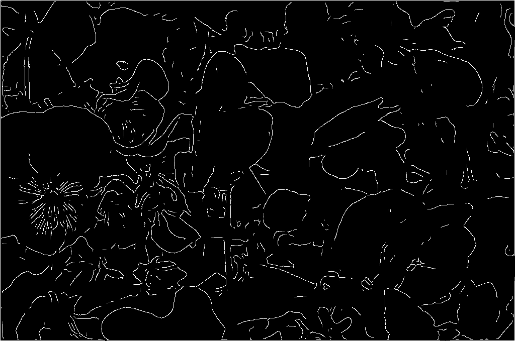
Below are three images. The first is the original image (converted to grayscale) and the others are the final results of running my implementation of the Canny edge detector with different settings, where white lines indicate an edge. It is not as obvious with this image, but different setting for the Gaussian blur and for the thresholds can produce drastically different results. You may have noticed that there are “edges” around the border of the image. This is because when I perform blurring I assume that the pixels outside the boundaries of the image are black, so the pixels at the border become darker, which causes a sharp gradient between the light flowers and the dark border.

Photometric Stereo

The final assignment was to implement photometric stereo, which is a technique for estimating the shape of an object based on several image of the object under differed lighting conditions. In contrast to the Canny Edge Detector, which was conceptually simple to understand but tricky to implement, photometric stereo was simple to implement but the underlying theory was difficult to understand. I will try to explain the implementation without getting into the details of why it works (which I still don’t fully understand). Unfortunately I am unable to provide the test images I used, but a quick search online should reveal numerous examples of how photometric stereo.

Photometric stereo requires at least three images of the same object from the same perspective, but with the light source coming from different directions. Given that information, there are several steps which will end with estimating the height map of the image. First you must find the albedo and surface normals of the image. Then with that information you can generate the height map.

Finding Albedo and Surface Normals

Albedo is also known as the reflection coefficient. It is a number between 0 and 1 that basically describes how much light is reflected by a surface. A perfectly black surface which reflects no light would have an albedo of 0 and a perfectly white surface would have an albedo of 1. The surface normal is a vector that is perpendicular to the surface at a given point. This is the information that gives you the shape of the object and allows you to estimate a height map.

Finding the albedo and surface normals requires some matrix math. We are given the information for two matrices S and I, where S is an N×3 and I is an N×1 matrix, where N is the number of images. Each row of S contains the coordinates of the light source direction for each image. Each row of I contains the intensity at a given pixel of each image, where the intensity is based on the grayscale value of the image, scaled from 0 to 1. Each row of both matrices is also multiplied by the intensity at a given pixel. This will eliminate any contribution from shadows, where the intensity would be 0.

Given those two matrices, you can calculate the surface description g, which is a 3-dimensional vector with a magnitude equal to the albedo and a direction equal to that of the surface normal. g is given by the following formula.

\( \textbf{g} = (\textbf{S}^T \textbf{S})^{-1} \textbf{S}^T \textbf{I} \)

Given the surface normal we can estimate the height of the object in the image at each point. Below are two formulas which you can use to find the depth at a point, given the surface normal at that point and the height at an adjacent point. I won’t go into detail about the derivation, but if you’re interested, you can read this.

\( z_{x, y} = z_{x-1, y} - \frac{n_x}{n_z} \\ z_{x, y} = z_{x, y-1} - \frac{n_y}{n_z} \)

Since we need the height at one point to derive the height at another, we start start by assuming the height at the top-left pixel is 0. The choice of both the pixel and the height is arbitrary.

Given the point at a single pixel, you can work your way throughout the image and find the height at every pixel. To do this, you must travel along a path from the starting pixel to each pixel. Again, the choice of this path is arbitrary, but it can affect your final result (since it is just an estimate). I chose to travel down then across to reach each pixel. To make your results more accurate, you could calculate the height based on several different paths and find the average calculated height.

Reflection

These programming assignments were a great exercise both in programming and in learning about computer vision. That is not to say that implementing random image processing algorithms is enough to teach you about computer vision, but it is a great supplement to help you to understand the concepts better.

If you are interested you can view the code on GitHub. I plan to (eventually) add examples and hopefully a few more features.